Last month I saw the bonkers $870M TypeSafe series A, and honestly was a little dumbfounded. I remember talking about this "safe LLM output" strategy a couple years ago, and the speedrun arrival of legitimately competitive clones mere days after release supported this idea that the problem was "not that insightful". Later, I realized their core bet wasn't necessarily "provide an accurate classifier", but probably more like "reduce MLE load" and "expand market for classification" thanks to implementation ease. Those insights came from me having built out taggit.io 7 years ago, a text classifier platform enabling anyone to train and use text classifiers. (alas, The Market Wasn't Ready™)
After going through the N stages of grief seeing something succeed spectacularly there (and coming out the other side), I realized that a) the scaled text classification problem was still interesting, b) the state of the art had moved since I last looked, and c) there was probably something interesting to explore at the intersection there. This post is a walk through that garden, narrating the space, my findings, and presenting a little demo.
tl;dr
- Decision models are essentially zero-shot classifiers. By capturing and labeling data, you can perform much better and much cheaper.
- A 4B fine-tune (a LoRA) achieves 0.91 macro F1 @ $6.10 per 1M decisions (vs 0.77 OpenAI @ $19.20 per 1M). A 33M classifier distilled from the LoRA achieves 0.894 macro F1 @ $0.09 per 1M. (evaluated on the taggit dataset)
- Decision on strategy is dominated by value of classifier accuracy vs volume. Most should prototype with the decision model, and plan for the capture + label loop as the product demonstrates value.
- calibrate.sao.dev demos how to do a labeling loop (label capture is private, model exports free)
Decision Models / Classifiers
The decision model, an LLM sampling output probabilities for one token to represent answer class, is essentially a zero-shot classifier. Traditionally, classifiers were trained from scratch on labeled data, learning everything they knew about the task from it. Later, for well-resourced domains (text, images, etc), we realized we could pre-train most of the network on unlabeled data, so a classifier starts out knowing the language and only has to learn the task: e.g. a pre-trained encoder with a logistic layer on top, still a very common text classifier recipe. I'd put the decision model at this spectrum's extreme: it relies entirely on what the pre-trained model already knows, plus the LLM's in-context learning to adapt to each problem.
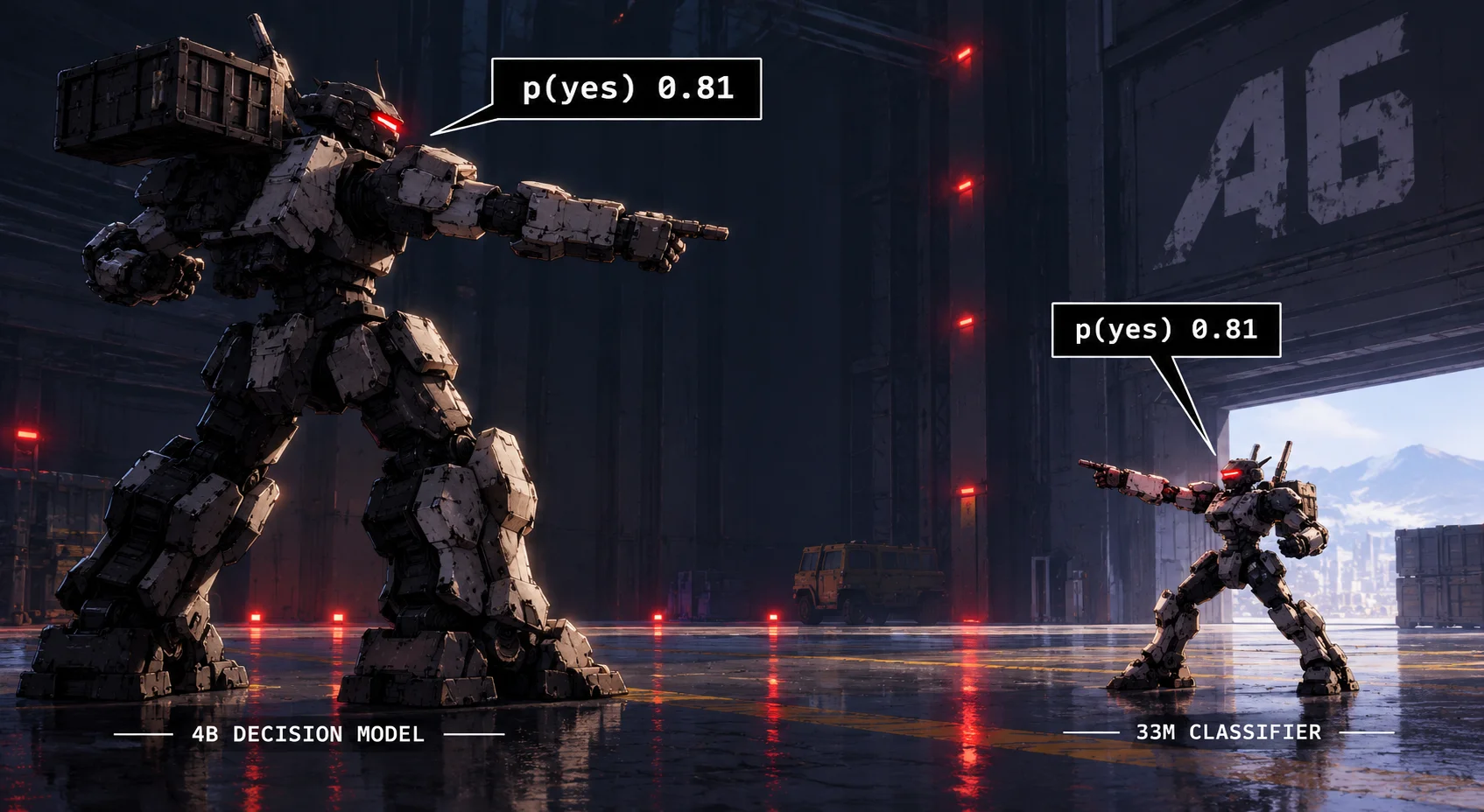
If you squint, the classifier fills an interesting role in our products and systems: it adapts a squishy, subjective domain into a simple categorical domain local to the formalisms of the business/product/etc. It turns arbitrary text into a "safety/trust risk" flag, or an image into "there is an apple at these coordinates". In a significant way, the ability to create, maintain, and improve classifiers is the ability to adapt a real-world problem into a software solution, and create a product around it.
On our path to discussing the right strategy per use case in the labels/classifiers/decision-model space, we're going to discuss some important concepts that support the decision:
- Accuracy is Incomplete - and the metrics you should be looking at for classifiers.
- Labels are Critical - the core roles that labeling plays in any system doing classification.
- Comparing Strategies - placing available strategies in the (setup cost, inference cost, classifier quality) space.
- Bootstrapping - decision models as the on-ramp to "real" classification systems.
- Demo - a working labeling loop you can use today: describe a classifier, label what it asks, export it as a container.
Accuracy is Incomplete
In classification, accuracy is a very incomplete metric, especially under class imbalance - and almost all classifiers have non-trivial class imbalance. If you're looking for vibes-similar quality metrics, you're probably looking for precision, recall, and F1 score; wikipedia has a great explainer for them. Borrowing their phrasing: Precision is the ratio of positively classified instances that were true positives: TP / (TP + FP); and Recall is the ratio all positive instances which were classified as positive: TP / (TP + FN). F1 score is the harmonic mean of precision and recall, a single number that's only high when both are. Every table in this post reports macro F1: the F1 of each class (here, "yes" and "no"), averaged, so a classifier can't score well by ignoring the rare class.
- ACCURACY
- 95%
- PRECISION
- —
- RECALL
- 0.00
- F1
- 0.00
- ACCURACY
- 93%
- PRECISION
- 0.40
- RECALL
- 0.80
- F1
- 0.53
Let's take 200 items where 10 are positive. A classifier that always says "no" is 95% accurate, but catches nothing: its macro F1 is 0.49. One that learns something and catches 8 of the 10 at the cost of 12 false alarms is less accurate at 93%, but its macro F1 is 0.75, and it's actually worth shipping. The taggit data in this post has the same shape: always answering with the majority class scores 0.61 accuracy, but 0.37 macro F1.
Another dimension missed by both accuracy and P/R/F1 is calibration. A classifier is calibrated when its confidence means what it says: of the answers it gives at 80%, about 80% are right. That's what makes a 0.54 useful rather than noise: you can route it to a person for review, auto-accept the 0.98s, and set those thresholds knowing what they'll cost you. (Calibrated doesn't mean often unsure; a very accurate model can put nearly everything near 0 or 1, and be right to.) To my pleasant surprise, people have actually been talking about calibration with decision models. In my experience building classifiers at magnificent-seven scale, consumers often "just want the answer"; the tide of ML education seems to be rising with LLMs.
The standard measure is Expected Calibration Error (ECE): group answers by confidence (say into 10 bins), compare each bin's average confidence to how often it was actually right, and average the gaps, weighted by how many answers fall in each bin. 0 is perfectly calibrated.
HOW ECE IS COMPUTED
Bin every prediction by its score, then compare each bin's average score to how often its items were truly yes. A calibrated classifier lands on the diagonal; ECE is the average gap, weighted by how many predictions fall in each bin.
Here's how the strategies in this post measure up on the taggit holdouts:
| Strategy | ECE | conf 0.5–0.6 | conf 0.6–0.7 | conf 0.7–0.8 | conf 0.8–0.9 | conf 0.9–1.0 |
|---|---|---|---|---|---|---|
| OpenAI decisions | 0.089 | 0.34 (440) | 0.58 (166) | 0.57 (195) | 0.73 (364) | 0.92 (2,506) |
| Decision model, zero-shot | 0.049 | 0.55 (441) | 0.68 (438) | 0.77 (565) | 0.93 (1,170) | 0.98 (1,057) |
| Embedding classifier | 0.016 | 0.57 (281) | 0.68 (325) | 0.77 (386) | 0.86 (584) | 0.96 (2,095) |
| Decision model, few-shot k=4 | 0.040 | 0.54 (267) | 0.75 (266) | 0.76 (378) | 0.91 (776) | 0.98 (1,984) |
| Distilled classifier | 0.031 | 0.59 (97) | 0.54 (71) | 0.69 (114) | 0.73 (226) | 0.96 (3,163) |
| Decision model, fine-tuned (LoRA) | 0.019 | 0.53 (75) | 0.61 (71) | 0.77 (94) | 0.76 (190) | 0.97 (3,241) |
Each cell is a bin's accuracy and, in brackets, how many of the 3,671 holdout labels fall in it, binned by the model's confidence in its own answer (the top option's probability, so never under 0.5). ECE is the gap between confidence and accuracy, averaged over bins weighted by their labels.
The models trained on labels are the calibrated ones (ECE 0.016–0.031). The zero-shot decision model is underconfident (right more often than it says), and OpenAI decisions are overconfident. So, two numbers: macro F1 for how often a classifier is right on both classes, and ECE for whether you can act on its confidence.
Labels are Critical
The really challenging part about classification in general is that once you really get into it, classification tasks can get very nuanced. Even a subtle change in phrasing can change the output class, and in ways even relatively high capacity decision models don't catch. Labeled data is the way to handle this: for many nuances of the classification, it is simply more effective to show than tell. In industrial labeling programs, human labelers are given both highly refined narrative text and instructive examples demonstrating nuances. The same is necessary for classifiers trained to solve the same problem.
Every strategy tested as part of this work (other than few-shot) improved with labels: (some more than others)
| Human labels | Models | embedding classifier | few-shot k=4 | LoRA | distilled classifier |
|---|---|---|---|---|---|
| 50 | 47 | 0.689 | 0.875 | 0.860 | 0.842 |
| 100 | 44 | 0.754 | 0.872 | 0.894 | 0.875 |
| 200 | 31 | 0.826 | 0.869 | 0.927 | 0.902 |
| 400 | 11 | 0.853 | 0.894 | 0.931 | 0.914 |
| all (83–1,201) | 47 | 0.821 | 0.872 | 0.912 | 0.894 |
Mean over the models with more training labels than n (44 at 100, 31 at 200, 11 at 400; all 47 otherwise), each tier given the model's latest n human labels and scored on the same holdout; at all labels, few-shot, LoRA and head are the headline rows. Rows are not one population: the larger counts are the better-labeled models.
The distilled classifier is the embedding classifier's 33M encoder fine-tuned on the n labels plus the n-label LoRA's probabilities for 4,000 nearby unlabeled spans.
Categorically, label sets fall into two purposes: improving the classifier, or measuring the classifier's quality metrics.
For improving the classifier, you want a base of representative data for the common cases/themes/etc, but you also want representation in the training set for the details that make the decision boundary complex. There are pockets of examples that are hard, but show the nuance from phrasing, word-sense disambiguation, etc. They have much higher impact on net classifier quality than another basic example does. You'd source examples to label for this purpose via different sampling strategies: random sampling, corrections by domain operators, and from low-confidence answers by your existing classifier (another reason calibration is important). These examples are not suitable for calculating the expected future performance of the model, though, since a) the sampling process doesn't match reality, and more seriously, b) they were chosen precisely because a classifier got them wrong (active learning), so they're harder than what the classifier will usually see.
This is one nit on the measurements in this blog post: the taggit data was labeled this way, so difficulty rises over time: later labels were chosen mostly because a classifier got them wrong. Since the evaluation holds out each model's latest labels, the quality numbers here are very likely underestimates.
For quality metrics, you want to construct a sampling process that produces a representative sample from your domain continuously, so you can have something label it (a human, or a higher capacity model if you're cheap), and then use those labels to identify quality regressions or performance holes. The world and language legitimately does change, and thus so does the data distribution - this is why no classifier over human-generated data is ever complete. You might choose to do stratified sampling to ensure fidelity across categories. Generally its worth a human being involved (at least in part) in the ongoing labeling loop, as it is generally where new classes of hard examples are identified.
There is essentially one case where you don't need a labeling loop set up, and that's the low-volume regime where vanilla decision models are accurate enough. This is a sweet spot where renting what a hosted decision model already knows makes a lot of sense. For essentially all other cases, you want a labeling loop:
- To assert continued classifier performance. (the domain drifts, the world changes!)
- To enable very high quality classifiers (in calibration and accuracy): even LoRAs of decision models need labels from the domain to learn the nuance of your task.
- To improve cost scalability: small models need many more labels to match a big one, or a big model to learn from. That's distillation: a model fine-tuned on your labels answers for lots of unlabeled text, and a small model learns to copy its answers.
Comparing Strategies
In my walk around the space I explored a few categories of strategies:
- Hosted decision models - OpenAI decisions (its Decisions API), zero-shot. No labels, no infra, pay per call.
- Open decision models - a 4B open model (h2o-lightning-4b) run zero-shot, few-shot (the nearest labeled examples in the prompt), or fine-tuned on the labels with a LoRA (a small set of trained weights added to the model).
- Embedding classifiers - a 33M pre-trained text encoder (bge-small) with a logistic layer trained on the labels. The encoder is frozen: only the small layer on top learns.
- Distilled classifiers - the same 33M encoder, fine-tuned end to end on the labels plus the LoRA's answers for 4,000 similar unlabeled spans. (distillation: generating labeling data from a teacher, here the LoRA)
Sorted by F1, the table reads as one lesson: model size sets the cost, and how much of the model learned your task sets the quality.
| Strategy | Model | Learns your task from | Cost / 1M | Macro F1 | vs LoRA (F1, cost) |
|---|---|---|---|---|---|
| OpenAI decisions | undisclosed, hosted | nothing (instructions only) | $19.20 billed | 0.766 | −0.146 F1, 3.1× cost |
| Decision model, zero-shot | 4B | nothing | $5.67 GPU | 0.814 | −0.097 F1, 0.93× cost |
| Embedding classifier | 33M | labels, last layer only | $0.09 CPU | 0.821 | −0.091 F1, 1/67× cost |
| Decision model, few-shot k=4 | 4B | its 4 nearest labels, in the prompt | $19.69 GPU | 0.872 | −0.040 F1, 3.2× cost |
| Distilled classifier | 33M | labels + the LoRA's answers, whole model | $0.09 CPU | 0.894 | −0.018 F1, 1/67× cost |
| Decision model, fine-tuned (LoRA) | 4B | labels, whole model (via an adapter) | $6.10 GPU | 0.912 | reference |
Orange is the best of each numeric column; for vs LoRA (F1 behind it, cost as a multiple of its) the least F1 given up under $1 per 1M. Click an F1 for accuracy, macro precision and recall. Few-shot neighbours come from the model's own training labels (median 283) and add 484 prompt tokens per decision. OpenAI refused 231 of 3,671 holdout labels, each scored as a uniform guess; on the rest it scores 0.808.
Distilled classifier is the embedding classifier's encoder fine-tuned end to end on the labels plus the LoRA's probabilities for 4,000 nearby unlabeled spans: 66 MB of weights per classifier, where the embedding classifier's layer is a few KB on a shared encoder.
Latency (p50): OpenAI decisions 132 ms (request wall time, 8 in flight); Decision model, zero-shot 24.2 ms (L4 batch throughput); Embedding classifier 3.58 ms (one unbatched decision, all threads); Decision model, few-shot k=4 81 ms (L4 batch throughput); Distilled classifier 7.44 ms (one unbatched decision, one core); Decision model, fine-tuned (LoRA) 26 ms (L4 batch throughput). These answer different questions and are not ranked.
Rates. OpenAI: $0.10 per 1M billed input tokens (decisions guide, checked 2026-10-10). GPU: measured L4 seconds at Modal's $0.000222/s (modal.com/pricing, checked 2026-10-11), GPU kept busy, steady state; each vLLM container start adds 260 s, $15.72 per 1M at this run's size. CPU: the embedding classifier is 6.9 ms per decision on one thread (Ryzen 9 7950X3D, 16 vCPU; its p50 above used all threads), so 6900 core-seconds per 1M at Modal's $0.0000131 per physical core-second (modal.com/pricing, checked 2026-10-17), memory excluded. The distilled classifier runs the same graph and is priced the same; its own export timed 7.44 ms, inside this box's run-to-run spread.
OpenAI's hosted model only reads instructions and scores lowest; a 33M model that learned the whole task from a teacher lands within 0.02 of the 4B LoRA at 1/67 of the cost. Plotting cost against quality, the frontier is short:
| Human labels | Strategy | Cost / 1M | Macro F1 | Frontier |
|---|---|---|---|---|
| 0 | majority | ~$0 | 0.372 | yes |
| 0 | zero-shot decision model | $5.67 | 0.814 | yes |
| 0 | OpenAI | $19.20 | 0.766 | |
| 50 | embedding classifier | $0.09 | 0.689 | |
| 50 | distilled classifier | $0.09 | 0.842 | yes |
| 50 | zero-shot decision model | $5.67 | 0.814 | |
| 50 | LoRA | $6.10 | 0.860 | yes |
| 50 | OpenAI | $19.20 | 0.766 | |
| 50 | few-shot k=4 | $19.69 | 0.875 | yes |
| all (83–1,201) | embedding classifier | $0.09 | 0.821 | |
| all (83–1,201) | distilled classifier | $0.09 | 0.894 | yes |
| all (83–1,201) | zero-shot decision model | $5.67 | 0.814 | |
| all (83–1,201) | LoRA | $6.10 | 0.912 | yes |
| all (83–1,201) | OpenAI | $19.20 | 0.766 | |
| all (83–1,201) | few-shot k=4 | $19.69 | 0.872 |
At 0 human labels the frontier runs majority (0.372 at ~$0), then zero-shot decision model (0.814 at $5.67).
At 50 human labels the frontier runs distilled classifier (0.842 at $0.09), then LoRA (0.860 at $6.10), then few-shot k=4 (0.875 at $19.69).
At all human labels (83–1,201) the frontier runs distilled classifier (0.894 at $0.09), then LoRA (0.912 at $6.10).
Mean over all 47 models, scored on the same holdouts (3,671 labels); OpenAI counts refusals as uniform guesses. Cost per 1M decisions: GPU rows are steady-state L4 seconds with the vLLM start excluded (260 s per container, $15.72 per 1M at these holdouts' size) and measured on the full holdouts, since a model's inference cost does not depend on how many labels trained it; the embedding and distilled classifiers (the same graph) are one CPU core at 6.9 ms per decision, OpenAI is billed. The distilled classifier learns from the LoRA trained on the same labels.
While it's tempting to construct a 2x2 here, the real process for non-MLEs (or busy MLEs) is to bootstrap with a decision model, then choose the strategy that best fits your requirements. If that's maximizing precision/recall, you're going to LoRA; for high scale at a reasonable price, it's a lower capacity model like the distilled classifier here, 0.02 F1 behind the LoRA at 1/67 of the cost (its cost moves to 66 MB of weights per classifier, and a LoRA to train as its teacher). Few-shot only makes the frontier at 50 labels, by a noise-sized margin, at three times the LoRA's price.
Bootstrapping
One thing that decision models get right as a product is giving you something useful from the get go. In the classic classifier paradigm, you need to label a bunch of data, write your text classifier software, host the model, and then you get to start making decisions based on its results and building the broader feature. With decision models, you literally just make an API call, and get something useful back. It's not the most accurate, but it proves feature value much sooner than a hand-built classifier.
Looking back on Taggit, I think this is actually a key insight: MLEs don't need help creating a classifier, they know how to do it already; non-MLEs who don't know how to create a classifier also don't have an intuition for when they are valuable, their costs, etc. This means they can't go from 0 to 1 in many cases, and can't know if the juice is worth the squeeze.
This makes the likely path for most recent adopters of decision models something like:
- Start with a hosted decision model. (If this meets your needs, you're done!)
- If you need to measure or improve quality, or significantly reduce cost, set up a labeling loop.
- If you need to improve classifier quality, fine-tune on your labels (a LoRA) before reaching for a bigger model: a model that learned your task beats a bigger one that only read the instructions.
- If you need to improve quality without increasing cost, you need to label more data.
- If you need to reduce cost, you need to use a smaller encoder. More labeling helps here, and distillation from a LoRA is a cheap way to boost performance.
calibrate.sao.dev
Having built a system like this before, I figured a demo would be helpful. There are two ways to try it:
- The extended demo at calibrate.sao.dev, where you can create your own classifier, bootstrap it, and use it.
- The embedded demo, where you can try out a small classifier I built out.
The purpose of the extended demo is to show that the labeling loop and bootstrapping part of building a classifier is actually not that much work, especially with a coding agent in the loop. Once you create a classifier, it will grill you with positive and negative examples, and then train an embedding classifier for you. (not the distilled one 1, to make hosting easier on me) You can then export this classifier as a docker image, allowing you to host inference on your own infra. Classifications also come with a correction link alllowing you to keep improving the classifier on calibrate.sao.dev if you want!
You can try out the in-browser example classifier for the app-crash topic from the taggit dataset:
A public classifier from the calibrate demo, run in your browser.
Doing this yourself with a coding agent should be pretty straight forward - just point it at this blog post and ask it to implement it for you.
Appendix
The data
| Dataset | |
|---|---|
| Models | 47 |
| Holdout labels (latest 20% per model) | 3,671 |
| Training labels (earliest 80%) | 14,781 in all; per model median 283, min 83, max 1,201 |
| Options per question | 47 binary |
| Majority-class baseline | accuracy 0.607, macro F1 0.372 |
By model name: 14 app-*, 7 clothing-*, 3 podcast-*, and 23 others (ad-annoyance, anger, anticipation, bad-service, checkout, cleanliness, …): app, product and podcast review complaints, service quality and sentiment. Each model is one human-labeled taggit question over a tagged span of review or customer text. Means are over models unless marked pooled. Text, label sources and per-label records live on the calibrate-systems share and are not summarised here.
- 47 taggit questions over review and customer text; binary; majority class 0.607 accuracy but 0.372 macro F1.
- Short spans of consumer-review English, labeled by one team. A multilingual or document-length task is a different benchmark; the ordering of strategies should hold, the numbers will not. Human labeled, before LLMs were a thing.
- Split by time (earliest 80% train, latest 20% holdout); holdouts are 20 to 300 labels per model, so per-model numbers are noisy and means over 47 are what to read.
Calibration and refusals
- ECE is pooled over all 3,671 holdout labels, in 10 bins of the model's confidence in its own answer. Per-model ECE at 20 labels is noise and is not quoted.
- The OpenAI row counts refusals as uniform guesses; answered-only it scores 0.808, still under the open 4B. Refusals are a real cost of a hosted decision model, so the full row is the fair one.
- The distilled classifier is calibrated within 0.03 (0.031 at all labels, 0.025 at 50): slightly overconfident, as its teacher is, and like its teacher more so on later labels. Rescaling its confidence with one temperature per classifier did not fix it: fit against the teacher, which had seen those labels, the temperature came out under 1 and sharpened it further.
What the costs mean
- Steady-state L4 seconds on Modal with the vLLM start excluded (260 s per container: $15.72 per million at this run's size, amortising to nothing at scale). Each tier is costed at its steady-state rate regardless of how many labels trained it; the 50-label runs measured higher because small holdouts batch badly, and that number predicts nothing.
- Modal's L4 rate matches AWS g6 on-demand; RunPod is about half, GCP a little under. The premium is billing shape (cold starts, idle), not the hourly rate.
- The embedding classifier is one CPU core at 6.9 ms per decision; its 3.58 ms latency in the table used every core. Latency is batch throughput for GPU rows and one unbatched decision for the embedding classifier; they answer different questions.
- Few-shot cost never amortises: every example is prefilled on every decision, which is why the LoRA wins at scale with the same labels.
- The distilled classifier runs the same graph as the embedding classifier and is priced the same ($0.09/1M), but costs 66 MB of weights per classifier (vs a few KB for the embedding classifier's layer on a shared encoder), ~$0.01 of L4 training, and ~$0.05 for its LoRA teacher.
The label curve
- Each size averages the models that have that many training labels: 47 at 50, 44 at 100, 31 at 200, 11 at 400, 47 at "all". The 400 column is the best-labeled models, which are also easier, so the "all" column dipping below it is selection, not labels hurting. Read within a column.
- Holdouts are 20 to 300 labels per model, so per-size differences under about 0.03 are noise.
How many nearest examples
| k | Macro F1 | ECE (pooled) | Prompt tokens / decision | GPU $ / 1M | p50 ms |
|---|---|---|---|---|---|
| 0 | 0.814 | 0.049 | not recorded | $5.67 | 24.2 |
| 4 | 0.872 | 0.040 | 484 | $19.69 | 81 |
| 16 | 0.879 | 0.039 | 1,567 | $65.20 | 267 |
Neighbours are each text's k nearest training labels by bge-small cosine, as prior chat turns, nearest last. GPU cost is steady state on an L4, latency batch throughput; every example is prefilled on every decision, so cost grows with k.
- 4 neighbours in the prompt buy 0.06 F1 over zero-shot; 16 buy 0.007 more for 3.3x the price. The elbow is early.
- Serving the LoRA with neighbours in the prompt did not beat the plain LoRA at these label counts.
Distillation and student capacity
- Distilling into the frozen embedding classifier (the teacher's answers train its logistic layer only) is a small lift: 0.03 over labels alone at 50 labels and 0.005 with all of them, on the 47. With no human labels, distilled from the zero-shot decision model, it scores 0.72 against its teacher's 0.81. The teacher at n labels is the LoRA trained on those n, labeling 4,000 unlabeled spans similar to the model's training text; an earlier version used the full-size LoRA at every n and read as flat from zero, which was the teacher leaking every label, not labels being unnecessary.
- A LoRA teacher's answers on those spans are nearly one-class (median 4.7% positive at 50 labels, against the zero-shot model's 16%), so pool selection needs class balancing before this does more.
- Fine-tuning the whole encoder on the same distillation is the big lift: +0.073 over the embedding classifier (0.894). The teacher's probabilities tie its hard answers on F1 (+0.002) but buy calibration (ECE 0.031 vs 0.047). Larger students do worse per dollar (ModernBERT-base 0.870, Qwen 0.8B 0.854).
- Why the frozen encoder stalls: the LoRA leads the embedding classifier by 0.05 accuracy, a 10x larger frozen encoder (bge-large) closes 0.016 of that, inside noise, and a nonlinear (MLP) layer 0.005. The encoder was trained for search, not your task, and frozen it can't change; letting it train closes 80% of the F1 gap.
- Not shown anywhere above: the bootstrap arms (spans OpenAI invents from the question, or multiplies from 50 judgments) ran on the 4 easy models only. Against the same 4 they are real gains (multiplied LoRA 0.928 vs 0.915 for a plain 50-label LoRA); rerun on all 47 before claiming them.